
6
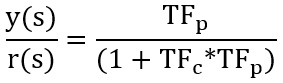
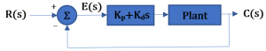
5.1 Control System Design for Feedback Systems
There are two classical design methods: Transient Response and Frequency Response. Frequency Response will be discussed in detail in Chapter 6.
Closed-Loop
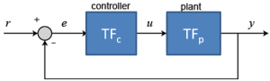
where e is error, TFc is the transfer function of the controller and TFp is the transfer function of the plant.
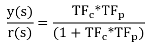
For a closed-loop:
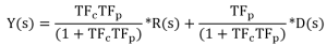
Closed-Loop with Disturbance

![]()
Alternate Feedback Systems
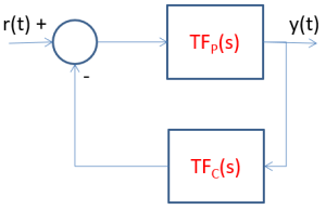
where TFP is transfer function of the plant and TFC is the transfer function of the controller.
Recall that the characterisic equation is the denominator of the transfer function set equal to zero, which in this case would be 1+TFCTFP=0.
Matlab Example 5.1: Solving for Possible Poles
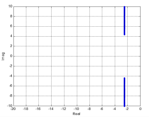
for K = 0:.1:1000
p = roots([1 5 (25+K)]);
plot(real(p),imag(p),’.’)
hold on
end
This code results in the following plot:
Next, we will obtain the plot using the rlocus function:
sys = tf(1,[1 5 25])
rlocus(sys)
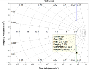
The rlocus function plots the root locus of the provided system (sys), allowing for us to view the pole trajectories as gain varies.
More information on rlocus can be found on the MATLAB website.
5.2 Root Locus Plots
A Root Locus Plot reveals all solutions of the characteristic equation for K > 0. The poles and zeros from an open loop transfer function can be plotted. The line represents the closed loop poles for gains of K=0, which occurs at the poles, to K=+∞.

General Rules for Root Locus
Rule #1: The poles of the closed loop system follow a path from the poles of the open loop system (K=0) to the zeros of the open loop system (or an asymptote):
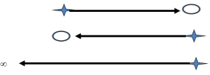
The open loop pole is a closed loop pole if K=0.
The open loop zero is a closed loop pole if K=∞.
Rule #2: Everything is symmetric across the real axis.
Steps to Construct a Root Locus Plot by hand
1. Locate and draw the poles and zeros of the open loop transfer function. Root locus diagrams will start at open-loop poles and end at zeros or infinity.
2. Determine the root loci on the real axis. Root loci exist on parts of the real axis where the total number of real poles and real zeros to the right of that part is odd.
![]()
If there are an odd number of poles and zeros on the real axis, the root loci will extend forever to the left after the last pole or zero as an asymptote of 180°.
If there are two poles or zeros at the same location, they should be counted as seperate entities.
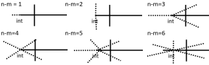
3. Determine asymptotes of root loci:
![]()
where n is the number of poles and m is the number of zeros.
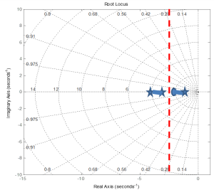
Asymptotes are drawn as lines from the point int:
![]()
Recall that these are always symmetric around the real axis.
If n-m=0, then there are no asymptotes.
For other cases:
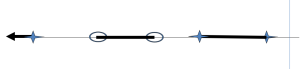
4. Find breakaway and break-in points:
Generally, on the real axis, if you have two poles or two zeros with a root locus between them, represented by a line connecting them, there is a break-in or breakaway point between them that must occur.
If the characteristic equation is described by B(s)+KA(s)=0 then

Solve to get a number of possible s values that will satisfy the above equation.
Only s values that appear on the root loci are break points. This can be determined by looking at the graph you have so far or by substituting the s back into B(s)+KA(s)=0 and solving for K. This must be positive for it to be a real break point.
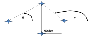
5. Determine the angle of departure and arrival.
If there is a complex pole, the root locus, represented by a line, will leave that pole in the direction known as the angle of departure. If there is a complex zero, the root locus will approach that zero at the angle of arrival. These can be calculated as needed.
Angle of departure from a complex pole = 180 – (sum of the angles of vectors to the pole from other poles) + (sum of the angles of vectors to the pole from all zeros)
Angle of arrival to a complex zero = 180 – (sum of the angles of vectors to the pole from other zeros) + (sum of the angles of vectors to the pole from all poles)
Example: AOD=180-(90+θ+Φ)
6. Find where the root loci cross the imaginary axis.
This can be achieved by substituting jw for s, equating the real and imaginary parts to zero and solving for K and w.
 where the poles are -1, -2 and -3.
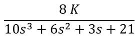
The closed-loop denominator is 1+KTFOLwoK=0=1+K/(s3+6s2+11s+6).
By substituting in jw for s,
(jw)3+6(jw)2+11jw+6+K=0 → -j(w)3-6w2+11jw+6+K=0
-6w2+6+K=0 and -j(w)3+11jw=0, so w=0, -3.3, 3.3 and K=-6, 60, 60.
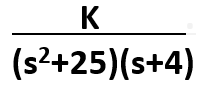
Example 5.1:
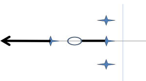
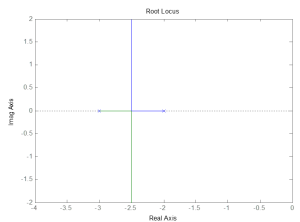
Step 1 and 2 for Root Locus:
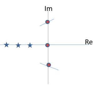
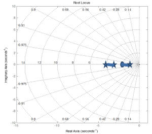
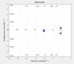
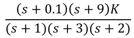
For the given transfer function, plot the Root Locus.

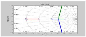
From the numerator, we see that a zero occurs at -2, as indicated by the hollowed circle symbol on the Root Locus plot, and poles occur at -1, -3 and -4, as indicated by the star symbols.
Step 3 for Root Locus:

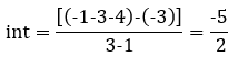
From our calculations, the asymptote occurs at -5/2 at a ±90° angle.
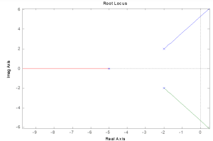
The same plot resulting from MATLAB is shown below:

Example 5.2:


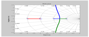
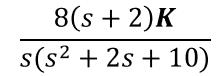
From the numerator of the transfer function, we can determine that the open loop zero is -10. From the denominator of the transfer function, we can determine that the open loop poles are -0.5 ± 0.866i. The zero and poles have been plotted below.
There are two poles and one zero, so n-m=1, resulting in one resulting asymptote at 180°.
There is only a zero on the real axis, so there is an odd number of poles and zeros on the real axis. This means that the root loci will extend forever to the left after the zero as an asymptote of 180°.
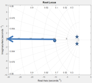
Next, we need to determine if the root locus crosses the imaginary axis. This can be achieved by substituting jw for s, equating the real and imaginary parts to zero and solving for K and w.
After substituting jw for s, this is our resulting transfer function: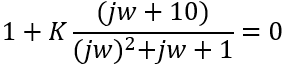

(jw)2 + (1+K)jw + (1+10K) = 0
Recall that j2 = -1, so our equation becomes -(w)2 + (1+K)jw + (1+10K) = 0
Next, we can reorder the equation so that the real terms come before the imaginary terms: (1+10K) – (w)2 + (1+K)jw=0
For the imaginary terms in the equation: (1+K)jw=0, so K=-1 or w=0.
For the real terms in the equation: (1+10K) – (w)2 = 0
If K=-1, then (1+10(-1))-(w)2=0, so -9 = (w2), so w is not real.
If w=0, then (1+10K)-0=0, so K=(-1/10) which is not positive.
There are no imaginary crossings.
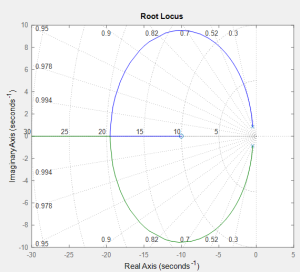
Lastly, we know that all lines must go from open loop poles to open loop zeros or asymptotes, and that everything is symmetric across the real axis. We know that there will be a break-in point between -10 and -∞.

The plot resulting from MATLAB is shown below:
MATLAB Example 5.2: 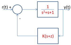
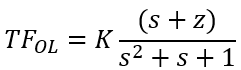
From the numerator of the transfer function, we can determine that the open loop zero is -z. From the denominator of the transfer function, we can determine that the open loop poles are -0.5 ± 0.866i.
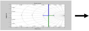
By entering this code into MATLAB, the poles are plotted on the Imaginary vs. Real plot:
sys = tf([1],[1 1 1]);
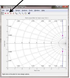
sisotool(sys)
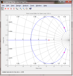
By clicking the o symbol as shown in the figure below, we can add a zero to the plot.
Recall that you can create the open loop system in MATLAB:
num = [1 2 3];
den = [ 1 2 3 4];
sys = tf(num,den);
or
k = 1;
z = [-1 -2 -3];
p = [-4 -5 -6];
sys = zpk(z,p,k);
and you can also use:
rlocus(sys)
or sisotool(sys)
SISOTOOL
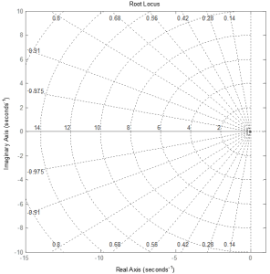
When you call sisotool(sys) in MATLAB, a Control System Designer window opens and the Root Locus Editor panel can be located.

You can import a system that describes your plant and you can get the root locus plot:
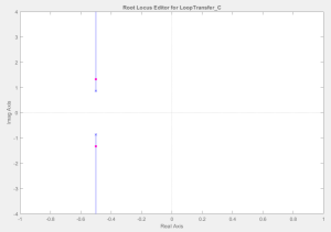
You can also use graphical tuning to change the display using “Tuning Methods” on the Toolbar.
You can add gridlines and design constraints to assist with selecting the best poles. By dragging the pink square, you can see what effect different gains may have. You can also add controller poles and zeros with the menu buttons.

5.3 Reshaping Root Locus
Some General Themes to Root Locus Design
Nearby zeros tend to shift the root locus towards the zero

Nearby poles tend to shift the root locus away from the pole
You can use zeros and poles to reshape your root locus!
Adding Poles and Zeros
1. Generally it is beneficial for settling time and overshoot to put a zero on the left, close to the root locus.
2. A controller that gives you a zero is a Proportional-Derivative Controller.
Controller=Kpr+Kds=K(s+z)
GH=K*TFplant*(s+z)
3. Another choice is a lead controller.
Controller=K(s+z)/(s+p)
GH=K*TFplant*(s+z)/(s+p)
5.4 Fixing Steady-State Error with a Controller
5.5 Steady-State Error
Exercises
Exercise 5.1
Given the open-loop transfer function, what is the characteristic equation?
1. 
2.
3.
Exercise 5.2

Write an algorithm to solve for poles at K from 0 to 25.
You might want to rearrange the equation to make it a polynomial.
Exercise 5.3
Construct the root loci by hand.
1. 
2. 
Exercise 5.4
Sketch the following root loci.
1.
2.
Exercise 5.5
How might we improve the transient response (settling time) of these root loci (a) with just changing proportional gain? What is the best 2% settling time possible?
1.
2.
Media Attributions
- chapter6_trend4
