
1
1.1 Why do we model systems?
Modeling allows one to analyze a system without actually constructing the physical system. It is not always ideal to analyze a physical system for various reasons, such as expense. Using differential equations, we are able to represent dynamic systems in mathematical terms in order to gain insight to its dynamic behavior.
For example, in mechanical systems, one can build such equations from the equations of motion:![]() , where F are the forces applied to the body, m is the mass of the body and a is the acceleration of the body with respect to the inertial frame, and
, where F are the forces applied to the body, m is the mass of the body and a is the acceleration of the body with respect to the inertial frame, and ![]() , where M are the moments applied about the center of mass of the body, I is the body’s moment of inertia, and α is the angular acceleration of the body. Similarly, one can use Kirchoff’s laws to build dynamic system equations for electrical systems.
, where M are the moments applied about the center of mass of the body, I is the body’s moment of inertia, and α is the angular acceleration of the body. Similarly, one can use Kirchoff’s laws to build dynamic system equations for electrical systems.
In this chapter and the next, we will examine two mathematical representations of dynamic systems: the state-space representation and the transfer function. In Chapter 3, we will then build the mathematical model of the dynamic behavior of mechanical, electrical, thermal, and fluid systems in these two forms.
1.2 State-Space Representation of Differential Equations
In control systems, state-space representation is a representation of a dynamic system that is achieved by breaking down high-order differential equations into multiple first-order differential equations.
The following terminology is important for understanding state-space representation:
State is the smallest set of variables (n) such that knowledge of the value of these variables at a given time (to) and knowledge of any system input determines the dynamic behavior of the system.
State variables are the variables making up the smallest set of variables determining the state of a system (x1, x2, x3,…xn).
A state vector is a vector of the state variables ( x ).
State-space is the n-dimensional space where the axes are the state variables. Any state can be represented as a point in this space.
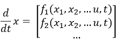
State-space equations are a set of equations modeling a dynamic system in state-space. In general these equations take the form:
To form the state-space representation, it is first important to obtain all the differential equations that describe the system. In Chapter 3, we will discuss how these may be derived. Once you have the differential equations that describe the dynamics of a system, the following steps can be used to create the state-space equations:
- Solve each differential equation for the highest derivative.
- If the highest derivative of an equation is greater than one, you will want to have another state variable for each order above one (so two state variables for a second-order differential equation for example). Create another differential equation for each order of the highest derivative. These equations should simply equate the derivative of one state variable to another state variable.
- Use these equations to create the state-space equations.
Example 1.1: From Differential Equation to State-Space Representation
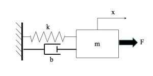 In this example, there is a mass-damper-spring system. There is an external force applied to the system, notated as F in the diagram. The spring and damper are assumed to behave linearly, friction is negligible, and mass is a point.
First, we must determine the differential equations that adequately describe the model. By applying ![]() , we determine that the external force applied is acting in the positive x-direction, while the spring and damper forces are acting in the negative x-direction, which is towards the wall.
, we determine that the external force applied is acting in the positive x-direction, while the spring and damper forces are acting in the negative x-direction, which is towards the wall.
The result is a second-order differential equation:![]()
Recall that x indicates position, ![]() indicates velocity and
indicates velocity and ![]() indicates acceleration.
indicates acceleration.
We will assign x, which is position, to variable x1 and ![]() , which is velocity, to variable x2:
, which is velocity, to variable x2:

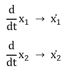
Next, we will take the derivative of x1 and x2:
Finally, we know that the resulting ![]() is velocity, which is equivalent to x2, and resulting
is velocity, which is equivalent to x2, and resulting ![]() is acceleration, which is equal to the rearranged second-order differential equation we found for the system:
is acceleration, which is equal to the rearranged second-order differential equation we found for the system:
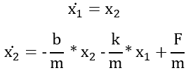
Writing this in matrix form becomes:
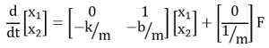
This is State-Space Representation.
Example 1.2: Inverted Pendulum
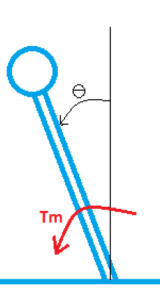
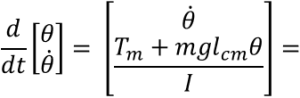
Below is the differential equation representing the motion of an inverted pendulum with an applied torque:
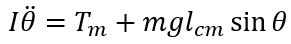
In Figure 1.1 of the inverted pendulum, Tm represents the applied torque. This system is not translating due to being fixed on one end. By applying ![]() , we can derive Equation 1.1. In addition to the applied torque, we have the moment created by the perpendicular force and the length of the string. Our state-space variables are θ and
, we can derive Equation 1.1. In addition to the applied torque, we have the moment created by the perpendicular force and the length of the string. Our state-space variables are θ and ![]() . Our state-space is 2-dimensional and the resulting state-space equations are:
. Our state-space is 2-dimensional and the resulting state-space equations are:
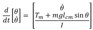
To solve the resulting differential equations, we need to know the initial conditions, and what input signals are being introduced to the system, which in this case would be Tm.
1.3 Solving State-Space Equations Numerically
With the state-space formatted differential equation, initial conditions of the state variables, and any input signals to the system, it is possible solve for the dynamics of the state variables with time.
Using Ordinary Differential Equation (ODE) Solvers, such as Runge-Kutta Methods, we can also use ODE Solvers through MATLAB. Information on ODE Solvers in MATLAB is available online.
Matlab Example 1.1
To implement a state space equation, we could use an ordinary differential equation (ODE) solver. These solvers use a numerical method to integrate the state space equations over time. To use Matlab’s ODE solvers, one first has to create a function representing the state-space equation. In this example, we will use the equation of a damped inverted pendulum.

%% This function is the state-space representation
% of an inverted pendulum
function xdot = pendulum(t, x)
% input variables: t for time,
% x is an array of the state variables:
% angle and angular velocity
xdot = x; % setting xdot is the same shape and size as x
%setting some constants
g = 9.8;
lcm = 1;
m = 1;
I = 1;
B = 1;
%State space equations. These equations return an array
% xdot that is the derivative of angle and angular velocity
xdot(1) = x(2); %dtheta/dt = theta_dot
xdot(2) = (m*g*lcm*sin(x(1))-B*x(2))/I;
end

We can also build these operations in one file using the @ to designate the function and adding the function to the end of the same file.
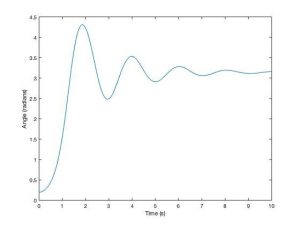
%% Call Ode Solver for the pendulum dynamic equations
th_0 = 0.2;
th_dot_0 = 0;
[t,x] = ode45(@pendulum_damped, [0 10], [th_0 th_dot_0]);
figure(1)
plot(t,x(:,1))
xlabel(‘Time (s)’)
ylabel(‘Angle (radians)’)
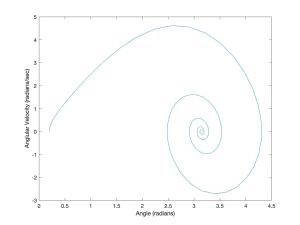
%% Phase plane plot
figure(2)
plot(x(:,1),x(:,2))
xlabel(‘Angle (radians)’)
ylabel(‘Anglular Velocity (radians/sec)’)
%% Call Ode Solver for the pendulum dynamic
% equations for several initial conditions
for th_0 = -6:1:6
for th_dot_0 = -6:1:6
[t,x] = ode45(@pendulum_damped, [0 10], [th_0 th_dot_0]);
figure(3)
plot(x(:,1),x(:,2))
xlabel(‘Angle (radians)’)
ylabel(‘Angular Velocity (radians/sec)’)
hold on
end
end
%% This function is the state-space representation
% of an inverted pendulum
function xdot = pendulum_damped(t, x)
% input variables: t for time,
% x is an array of the state variables:
% angle and angular velocity
xdot = x; % just making sure xdot is the same shape and size as x
%setting some constants
g = 9.8;
lcm = 1;
m = 1;
I = 1;
B = 1;
% State space equations. These equations return
% an array xdot that is the derivative of angle and
% angular velocity
xdot(1) = x(2); %dth/dt = th_dot
xdot(2) = (m*g*lcm*sin(x(1))-B*x(2))/I;
end
1.4 Linearization
Through the process of Linearization, a nonlinear model is represented as a linear model through use of linear approximation.
Taylor Series Expansion
In order to perform Linearization, the first two terms of the Taylor Series Expansion can be used.
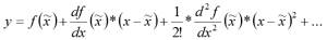
where ![]() is the nonlinear equation,
is the nonlinear equation, ![]() is the equilibrium point, and x is the state variable of the system
is the equilibrium point, and x is the state variable of the system
The resulting y equation is the linear approximation for the nonlinear equation. The following example will detail the linearization process using Taylor Series Expansion.
Example 1.5 Linearization of sin(θ)
Problem Statement: linearize y=sin(θ) at ![]()

These are the first two terms of the Taylor Series Expansion

For the first term, we are able to plug in the value of ![]() into our nonlinear equation.
into our nonlinear equation.
For the second term, we take the derivative of the nonlinear equation and plug in ![]() into this equation.
into this equation.
![]()
Lastly, we sum the first and second term.
The result is the linear approximation of the nonlinear equation.
The following example is a continuation of Example 1.2 Inverted Pendulum with applied linearization.
Example 1.6: Linearizing an Inverted Pendulum with Applied Torque
Recall from Example 1.2, we have the resulting state-space equations shown above. If we linearize and assume that sinθ=θ then the equations become:
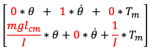
 Notice that the syntax of our state-space equations varies from the syntax of the equations we found at the end of Example 1.2.
Why can we express our equations in this syntax?
Recall that state-space equations take the form
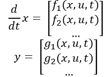
with the state variables vector expressed as x, the input variables vector is expressed as u and the output variables vector is expressed as y.
If the equations are linear, you can arrange the variables in the following way:

As long as these equations are linear and time invariant, A, B, C and D are matrices of constants.
Example 1.7: Cruise Control
Problem Statement: Determine the state-space equations for the cart in the figure.
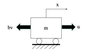
Cruise control is used in cars to maintain a certain speed despite disturbances such as changes in road conditions, elevation or resistance.
In this diagram, u represents the force exerted by the vehicle to advance forward and maintain the desired speed, and bv represents the resistive forces acting against u, such as wind resistance and friction between the tires and the road. The car’s position is x and its velocity is v.
In this problem, the variables are x, v, and u. The constants are b and m, with b representing a damping coefficient and m representing the mass of the car. The state is 2-dimensional.
Using![]() , we can determine that the system equation is
, we can determine that the system equation is ![]() . The state-space variables are x and v. The resulting state-space equations are:
. The state-space variables are x and v. The resulting state-space equations are:
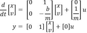
The resulting y equation above reflects our interest in controlling the speed of the car, so therefore we are interested in the velocity of the car.
Exercises
Exercise 1.1

Determine the differential equations that adequately models this system. List your assumptions. Then, represent the system in State-Space representation.
Exercise 1.2 Linearization of cos(θ)
Problem Statement: linearize y=cos(θ) at ![]() =π/2
=π/2
Exercise 1.3 Linearization of x2
Problem Statement: linearize y=x2 at ![]() =1
=1
