
4
3.1 Mechanical Systems
We will focus on systems that we can model as either translating or rotating rigid bodies.
Recall that the equations of motion for Mechanical Systems are![]() , where F are the forces applied to the body, m is the mass of the body and a is the acceleration of the body with respect to the inertial frame, and
, where F are the forces applied to the body, m is the mass of the body and a is the acceleration of the body with respect to the inertial frame, and ![]() , where M are the moments applied about the center of mass of the body, I is the body’s moment of inertia, and α is the angular acceleration of the body.
, where M are the moments applied about the center of mass of the body, I is the body’s moment of inertia, and α is the angular acceleration of the body.
One common assumption for modeling mechanical systems is that springs and dampers behave linearly. Recall that for a spring F = K * x where F is the spring force, K is the stiffness of the spring and x is the change in length of the spring from neutral. This is Hooke’s Law.

The simulation below demonstrates Hooke’s Law:
For dampers, the resulting equation is F = B*dx/dt where F is the force and B is the damping cofficient.

Tips for Solving
- Create a Free Body Diagram of each rigid body. This should create one second-order equation of motion for each direction of motion of the body (degree of freedom).
- If non-linear terms exist, consider if you can linearize them once you have the equations of motion.
- For state space, your variables will generally be the position and velocity terms for each degree of freedom of each rigid body.
For more complex mechanical systems, systems can sometimes be simplified by modeling them as a bunch of smaller rigid bodies connected by springs and dampers (a lumped parameter model).
Example 3.1: Mass-Spring-Damper System Review
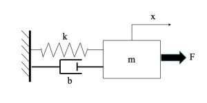
In this example, there is a mass-damper-spring system. There is an external force applied to the system, notated as F in the diagram. The spring and damper are assumed to behave linearly, friction is negligible, and mass is a point.
First, we must determine the differential equations that adequately describe the model. By applying ![]() , we determine that the external force applied is acting in the positive x-direction, while the spring and damper forces are acting in the negative x-direction, which is towards the wall.
, we determine that the external force applied is acting in the positive x-direction, while the spring and damper forces are acting in the negative x-direction, which is towards the wall.
The result is a second-order differential equation:![]()
Recall that x indicates position, ![]() indicates velocity and
indicates velocity and ![]() indicates acceleration.
indicates acceleration.
We will assign x, which is position, to variable x1 and ![]() , which is velocity, to variable x2:
, which is velocity, to variable x2:

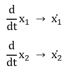
Next, we will take the derivative of x1 and x2:
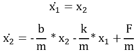
Finally, we know that the resulting ![]() is velocity, which is equivalent to x2, and resulting
is velocity, which is equivalent to x2, and resulting ![]() is acceleration, which is equal to the rearranged second-order differential equation we found for the system:
is acceleration, which is equal to the rearranged second-order differential equation we found for the system:
Writing this in matrix form becomes:
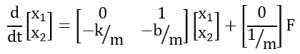
This is State-Space Representation.
Series and Parallel in Mechanical Systems
For components in Mechanical Systems that are in series, the force is equal for the components, and the displacement and velocity are summed for the components.

F = F1 = F2
x = x1 + x2
If Fi = Ki*xi then K1*x1 = K2*x2 = F
x=F/K1 + F/K2
Ktotal=(K1*K2)/(K1+K2)

F = F1 = F2
v = v1 + v2
If Fi = Bi*vi then B1*v1 = B2*v2 = F
v=F/B1 + F/B2
Btotal=(B1*B2)/(B1+B2)
For components in Mechanical Systems that are in parallel, the displacement and velocity are equal for the components, and the force is summed for the components.

F = F1 + F2
x = x1 = x2
If Fi = Ki*xi then K1*x1 + K2*x2 = F
Ktotal= K1+K2

F = F1 + F2
v = v1 = v2
If Fi = Bi*vi then B1*v1 + B2*v2 = F
Btotal= B1+B2
3.2 Electrical Systems
Recall the following equations necessary to model Electrical Systems:
- Kirchoff’s Current Law: the sum of currents leaving a node equals the sum of currents entering the node
- Kirchoff’s Voltage Law: the algebraic sum of all voltages around a closed path is zero
If the circuit interacts with an ideal DC motor, we use the equations ![]() where Kt is a constant, i is the current and T is torque, and
where Kt is a constant, i is the current and T is torque, and  where e is the effort/voltage and Ke is a constant.
Kt and Ke are generally considered equal in SI units.
When addressing electrical systems, you can think of it in terms of mechanical equivalents: current is equivalent to flow rate and voltage is equivalent to pressure.
Series and Parallel in Electrical Systems
Note that these differ from that of Mechanical Systems.
For components in Electrical Systems that are in series, the current is equal for the components, and the voltage is summed for the components.
V = F1 + F2
i = i1 = i2
V=R1 i + R2 i
Rtotal=R1 + R2
For components in Electrical Systems that are in parallel, the voltage is equal for the components, and the current is summed for the components.
V = V1 = V2
i = i1 + i2
V = R1*i1 = R2 *i2
i=V/R1 + V/R2
Rtotal=(R1*R2)/(R1+R2)
| System Type | Resistance | Capacitance | Inductance |
|---|---|---|---|
| Electrical | Symbol: R
V = i * R |
Symbol: C
V = (1/C) ∫ i dt |
Symbol: L
V = L di/dt |
| Mechanical | Damping (Ns/m)
F = B * v F= B dx/dt |
Stiffness (N/m)
F = K ∫ v dt F = K * x |
Mass (Ns2/m)
F = M dv/dt F = M d2x/dt2 |
| Rotational Mechanical | Damping (Nms/rad)
M = B * ω M = B dθ/dt
Energy Loss |
Stiffness (Nm/rad)
M = K ∫ ω dt M = K * θ
Stiffness is essentially the inverse of Capacitance Potential Energy Storage |
Inertia (Nms2/rad)
M = I dω/dt M = Id2θ/dt2
Kinetic Energy Storage |
Common Electrical Elements
Resistors
Recall that for a resistor ![]()
where e is the voltage and i is the current.
Inductance
Recall that for an inductor 
where e is the voltage and i is the current.
Capacitance
Recall that for a capacitor
where e is the voltage and i is the current.
Op-amps
Motors – DC, stepper, servo
Sensors – Tachometer, potentiometer, accelerometer, gyroscope
Tachometer: vt=K*w
Potentiometer: vp= vi/L x or vp=vi/L theta
Accelerometer: Va(s)/X(s)=(-ms2)/(ms2+cs+k) voltage typically proportional to linear acceleration for low frequencies (<< sqrt(k/m))
Gyroscope: voltage is typically proportional to rotational velocity
Feedback Controllers
| System Type | Resistance | Capacitance | Inductance | Effort | Flow |
|---|---|---|---|---|---|
| Electrical | Symbol: R
V = i * R |
Symbol: C
V = (1/C) ∫ i dt |
Symbol: L
V = L di/dt |
Voltage (V or e) | Current (i) |
| Mechanical | Damping (Ns/m)
F = B * v F= B dx/dt |
Stiffness (N/m)
F = K ∫ v dt F = K * x |
Mass (Ns2/m)
F = M dv/dt F = M d2x/dt2 |
Force | Velocity |
| Rotational Mechanical | Damping (Nms/rad)
M = B * ω M = B dθ/dt
Energy Loss |
Stiffness (Nm/rad)
M = K ∫ ω dt M = K * θ
Stiffness is essentially the inverse of Capacitance Potential Energy Storage |
Inertia (Nms2/rad)
M = I dω/dt M = Id2θ/dt2
Kinetic Energy Storage |
Moment | Rotational Velocity |
Example 3.2: Motor Position
Physical setup
A common actuator in control systems is the DC motor. It directly provides rotary motion and, coupled with wheels or drums and cables, can provide translational motion. The electric equivalent circuit of the armature and the free-body diagram of the rotor are shown in the following figure.

For this example, we will assume the following values for the physical parameters. These values were derived by experiment from an actual motor in Carnegie Mellon’s undergraduate controls lab.
(J) moment of inertia of the rotor 3.2284E-6 kg.m^2
(b) motor viscous friction constant 3.5077E-6 N.m.s
(Kb) electromotive force constant 0.0274 V/rad/sec
(Kt) motor torque constant 0.0274 N.m/Amp
(R) electric resistance 4 Ohm
(L) electric inductance 2.75E-6H
In this example, we assume that the input of the system is the voltage source ( ) applied to the motor’s armature, while the output is the position of the shaft (
 ). The rotor and shaft are assumed to be rigid. We further assume a viscous friction model, that is, the friction torque is proportional to shaft angular velocity.
System equations
In general, the torque generated by a DC motor is proportional to the armature current and the strength of the magnetic field. In this example we will assume that the magnetic field is constant and, therefore, that the motor torque is proportional to only the armature current  by a constant factor
  as shown in the equation below. This is referred to as an armature-controlled motor.
 (1)
(1)
The back emf,  , is proportional to the angular velocity of the shaft by a constant factor
  .
.
(2)
In SI units, the motor torque and back emf constants are equal, that is,  ; therefore, we will use
  to represent both the motor torque constant and the back emf constant.
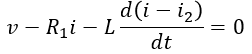
From the figure above, we can derive the following governing equations based on Newton’s 2nd law and Kirchhoff’s voltage law.
 (3)
(3)
 (4)
(4)
1. Transfer Function
Applying the Laplace transform, the above modeling equations can be expressed in terms of the Laplace variable s.
(5)
(6)
We arrive at the following open-loop transfer function by eliminating I(s) between the two above equations, where the rotational speed is considered the output and the armature voltage is considered the input.
(7)![$$ P(s) = \frac { \dot{\Theta}(s) }{V(s)} = \frac{K}{(Js + b)(Ls + R) + K^2} \qquad [\ \frac{rad/sec}{V} \ ] $$](http://ctms.engin.umich.edu/CTMS/Content/MotorPosition/System/Modeling/html/MotorPosition_SystemModeling_eq10498536974787467025.png)
However, during this example we will be looking at the position as the output. We can obtain the position by integrating the speed, therefore, we just need to divide the above transfer function by s.
(8)![$$ \frac {\Theta(s)}{V(s)} = \frac{K}{s ( (Js + b)(Ls + R) + K^2 )} \qquad [ \frac{rad}{V} ] $$](http://ctms.engin.umich.edu/CTMS/Content/MotorPosition/System/Modeling/html/MotorPosition_SystemModeling_eq13673943605533106994.png)
2. State-Space
The differential equations from above can also be expressed in state-space form by choosing the motor position, motor speed and armature current as the state variables. Again the armature voltage is treated as the input and the rotational position is chosen as the output.
(9)![$$ \frac{d}{dt}\left[\begin{array}{c} \theta \\ \ \\ \dot{\theta} \\ \ \\ i \end{array} \right] = \left [\begin{array}{ccc} 0 & 1 & 0 \\ \ \\ 0 & -\frac{b}{J} & \frac{K}{J} \\ \ \\ 0 & -\frac{K}{L} & -\frac{R}{L} \end{array} \right] \left [\begin{array}{c} \theta \\ \ \\ \dot{\theta} \\ \ \\ i \end{array} \right] + \left [\begin{array}{c} 0 \\ \ \\ 0 \\ \ \\ \frac{1}{L} \end{array} \right] V$$](http://ctms.engin.umich.edu/CTMS/Content/MotorPosition/System/Modeling/html/MotorPosition_SystemModeling_eq15318205225766984004.png)
(10)![$$ y = \left[ \begin{array}{ccc}1 & \ 0 & \ 0 \end{array} \right] \left [\begin{array}{c} \theta \\ \ \\ \dot{\theta} \\ \ \\ i \end{array}\right] $$](http://ctms.engin.umich.edu/CTMS/Content/MotorPosition/System/Modeling/html/MotorPosition_SystemModeling_eq04857532121070694232.png)
Attribution: “DC Motor Position: System Modeling”, by Messner et al. is licensed under CC BY-SA 4.0
Example 3.3

i=i1 +i2


3.3 Thermal Systems
When working with Thermal Systems, usually the equations will follow this format:
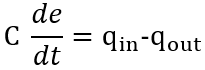
where e represents the effort variable, such as temperature or pressure, and q represents the flow variable, such as heat flux, fluid flow rate or current.
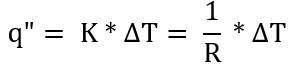
Recall that heat flux (q”) can occur through means of conduction, convection and radiation.
For conduction,![]() where k is thermal conductivity and L is the distance of conduction.
where k is thermal conductivity and L is the distance of conduction.
For convection,![]() where h is the convection heat transfer coefficient.
where h is the convection heat transfer coefficient.
For radiation,![]() where ε is emissivity and σ is the Boltzmann constant.
where ε is emissivity and σ is the Boltzmann constant.
For conduction and convection, q” is proportional to the temperature difference:
The equation for thermal capacitance, which is the insulating capacity of a material, is C = m * c where C is thermal capacitance, m is the mass measured in kg, and c is the specific heat of the material measured in kcal/kg ºC.
While heat transfer books use q” for heat flow rates, it is easier for us to consistently use just q, so it is the same as fluid flow problems.
Example 3.4
Determine the equation that models the system. Walls have resistance R and the outside temperature is Ta.

Based on Equation 3.1, we can determine that![]()
Heat is flowing out of the system, which explains why heat flow is negative for all instances.
Based on Equation 3.2, we can determine that T – Ta = qi * Ri
By substituting our second resulting equation into our first, we yield our final equation for this system:![]()
| System Type | Resistance | Capacitance | Inductance | Effort | Flow |
|---|---|---|---|---|---|
| Electrical | Symbol: R
V = i * R |
Symbol: C
V=(1/C) ∫ i dt |
Symbol: L
V = L di/dt |
Voltage (V or e) | Current (i) |
| Mechanical | Damping (Ns/m)
F = B * v F= B dx/dt |
Stiffness (N/m)
F = K ∫ v dt F = K * x |
Mass (Ns2/m)
F=M dv/dt F=M d2x/dt2 |
Force | Velocity |
| Rotational Mechanical | Damping (Nms/rad)
M = B * ω M = B dθ/dt
|
Stiffness (Nm/rad)
M = K ∫ ω dt M = K * θ
|
Inertia (Nms2/rad)
M = I dω/dt M = Id2θ/dt2
|
Moment | Rotational Velocity |
| Thermal | Resistance
walls
Energy Loss |
Capacitance
thermal masses
Potential Energy Storage |
|
Temperature | Heat Flux |
3.4 Fluid Systems: Incompressible Fluids
Recall that an incompressible fluid is a fluid that has is considered to have constant density, such as water.
Like Thermal Systems, when working with Fluid Systems, usually the equations will follow this format:
![]()
Capacitance in Incompressible Fluid Systems
In the figure, there is a cylindrical tank that contains an incompressible fluid.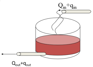
Qin+qi and Qout+qout are volume flowrates, so we know the following to be true: 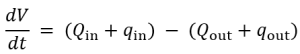
The capacitance is equal to the cross-sectional area of a cylinder, so the equation above becomes: ![]()
At steady-state, Qin = Qout, so 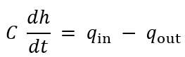
Recall that p=ρgh. We know that ρ and g are constants.
Our resulting equation is 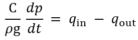
Resistance
For thermal systems with acting conduction or convection, q=(Tin-Tout)/R.
For fluid systems, which are linearized if turbulent, q=(Pin-Pout)/R.
For electrical systems, i=(Vin-Vout)/R.
Resistance in Fluid Systems
Recall the equation for Reynold’s Number (Re), a dimensionless number, that characterizes fluid flow as laminar or turbulent.
Re = ρVL/μ where ρ is the density of fluid, V is the velocity, L is the characteristic length and μ is the viscosity of the fluid.
For flow to be considered laminar, Re < 2100. When flow is laminar, you can use Poiseuille’s law:
Q = (πr4Δp)/(8μ*le)
where Q is the volume flow rate (m3/s), r is the radius, Δp is the pressure difference, le is the pipe length and D is the diameter. We also know that Q=πr2V.
For flow to be considered turbulent, Re > 2100. In this case, we can use the Darcy Weisbach equation:
![]()
where ƒ is the friction factor based on the Reynold’s number, wall roughness of the pipe, and the diameter, le is the pipe length, D is the diameter, ρ is the density of fluid, and V is the velocity. If we plug in Q=πr2V to the Darcy Weisbach equation, it becomes:
![]()
How can we model this for Control Systems?
We can represent pressure difference by the difference in heights of two reservoirs, known as the head difference.
P1 = ρgH1 and P2 = ρgH1 → Δp = ρg(H2-H1)
For Laminar flow, Q = constant Δp = ΔH/R
where R is the resistance (a function of pipe size and
fluid properties)
For Turbulent flow, Q = constant (Δp)1/2 = ΔH 1/2 K
where K is a constant
Example 3.6: Two-Tank Fluid Flow System

You have devised a way to water your sunflowers without even leaving the house! From your bedroom window, you use a hose to supply water to a two-tank system.
win represents the mass flowrate into Tank 1. The fluid flows into Tank 1, out of Tank 1 into Tank 2, and out of Tank 2. wout represents the mass flowrate out of Tank 2.
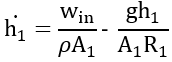
First, we will start by analyzing Tank 1. First, we have our equation based on fluid continuity:
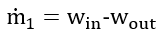
Where m is the mass of the fluid in the Tank 1 and win and wout are the mass flowrates in and out of the Tank 1.
Recall the following equations:


By substituting Equation 2 and 3 into Equation 1, we get: 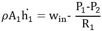
We know that P2, the pressure outside the tank, equals 0 due to being at atmospheric pressure, so: 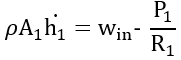
And by plugging in Equation 4 for P1, our equation becomes: 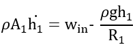
After rearranging, our equation becomes:
For analyzing Tank 2, we again start our equation based on fluid continuity: ![]()
Recall that wout of Tank 1 is win for Tank 2, so 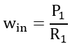
By substituting in Equation 2 and 3, our equation becomes 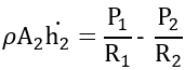
And by plugging in Equation 4 for P1 and P2, our equation becomes 
Rearranging and simplifying, the final equation becomes:
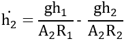
These resulting differential equations can be written in state-space form, as shown below:

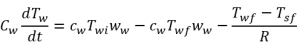
Flow through a Tank with Heat Transfer
![]()
![]() where fin and fout are heat flux, and C is thermal capacitance.
where fin and fout are heat flux, and C is thermal capacitance.
fout = qin*c*T
fin = qout*c*Tin
Where q is the mass flow rate, c is the specific heat of the fluid, and T is temperature.
If qin does not equal qout, then C could vary.
Example 3.7: Heat Exchanger
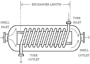
What differential equations can be used to model this system? We are interested in the temperature of the fluids.
![]() where fin and fout are heat flux, and C is thermal capacitance.
where fin and fout are heat flux, and C is thermal capacitance.
Recall heat flux by mass flow can be represented as f=w*c(Tin-Tout) where w is mass flowrate and c is specific heat.
For water:![]()
For steam: 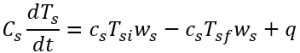
Knowing that![]()
Our resulting equations are:
![]()
3.5 Fluid Systems: Compressible Fluids
Capacitance in Compressible Fluid Systems
In the figure, there is a cylindrical tank that contains a compressible fluid, such as air.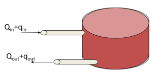
With compressible fluids, density is not a constant and varies based on pressure.
![]()
At steady-state, Qin = Qout, so ![]()
| System Type | Resistance | Capacitance | Inductance | Effort | Flow |
|---|---|---|---|---|---|
| Electrical | Symbol: R
V = i * R |
Symbol: C
V=(1/C) ∫ i dt |
Symbol: L
V = L di/dt |
Voltage (V or e) | Current (i) |
| Mechanical | Damping (Ns/m)
F = B * v F= B dx/dt |
Stiffness (N/m)
F = K ∫ v dt F = K * x |
Mass (Ns2/m)
F=M dv/dt F=M d2x/dt2 |
Force | Velocity |
| Rotational Mechanical | Damping (Nms/rad)
M = B * ω M = B dθ/dt
|
Stiffness (Nm/rad)
M = K ∫ ω dt M = K * θ
|
Inertia (Nms2/rad)
M = I dω/dt M = Id2θ/dt2
|
Moment | Rotational Velocity |
| Hydraulic | Resistance
valves, pipe flow
|
Capacitance
tanks |
Pressure | Flow rate | |
| Pneumatic | Resistance
valves, pipe flow
|
Capacitance
tanks |
Pressure | Flow rate | |
| Thermal | Resistance
walls
Energy Loss |
Capacitance
thermal masses
Potential Energy Storage |
|
Temperature | Heat Flux |

3.6 Modeling
Why are models useful?
Models allow for us to simplify the system into understandable and solvable terms. We can also compare systems and understand interactions. They can be used to predict behavior in other conditions.
For example, we may want to model a person sitting in a car as the following:
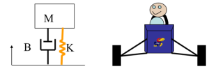
While this obviously does not perfectly model a person sitting in a car, this model may give us valuable insight into how a person might move and makes it possible to design systems around the person, such as a control system.
What do we need to consider when creating models?
Are the assumptions made reasonable?
Are the values used, such as weight or velocity, reasonable?
Can the model be validated by measurement?
Can the model be extrapolated to the desired scenario?
Example 3.8 : Record Player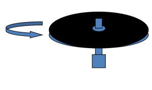
Input: Battery Voltage
Output: Record Speed
What do I know?
Voltage → Motor Speed → Record Speed
Use Circuits and Dynamics to get motor specifications:
Circuits: solve the equation of the circuit using Kirchoff’s Laws
Motor: ![]() and V = K * ωm
and V = K * ωm
Model the transfer of energy from the mechanical to electrical using an “ideal” motor.
Dynamics: solve the free body diagram of the spinning disc using Newtonian mechanics
Modeling Process Overview

The flowchart represents a simplified Process of Modeling. First, we must identify the real world system that we are looking to model. Once we have determined this, we can develop the Mathematical Model, which are the equations that are needed to develop the system and perform the desired analysis of this system. Next, we develop the Computational Model which is the algorithm based on the mathematical model, which can be developed in a software like MATLAB.
The process of Validation is assessing the computational model’s ability to make accurate predictions for our system. This can be done by comparing the outcomes of the computational model to experimental outcomes. Are the results reasonable and comparable? If not, why is this?
Throughout the modeling process, Verification processes should be performed. You may ask yourself the following questions:
Does the computational model accurately reflect our mathematical model? If not, is there an error in the algorithm that needs to be corrected? Are our results comparable to the results of a known problem with known solutions? If not, why is this?
Without Verification and Validation, we cannot say with confidence that our model can accurately make predictions for our system.
Errors in Modeling
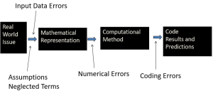
When developing a model, different errors can be introduced that we must be aware of.
Input Data Errors
When converting a physical system to mathematical representation, often times we need to make assumptions or simplifications. In these circumstances, we need to ensure that the assumptions and simplifications are reasonable. We must consider why these assumptions and simplifications are being made, and how they will affect the outcome.
Neglected Terms
Numerical Errors can also occur. These can be introduced based on the precision of a calculation or a rounding error.
In the numerical algorithm, coding errors may be introduced, especially if the algorithm is lengthy or complex. This could involve a typographical error or an error in syntax, which could lead to inaccurate results.
Exercises
Exercise 3.1: Spinning Disc
A disk is spinning on a viscous fluid at a rotational velocity w in a small electronic device. The angular position of the disk (θ) is an output that is used in the electronic device. A torque input acts on the rotating disk which has a rotational inertia of I.
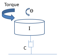 What is the equation of motion for the system?
What is the transfer function (θ(s)/T(s))?
What is the state-space representation of this system?
Exercise 3.2: Spring-Mass-Damper System
 Assume output is the position of M2.
Variables:
System Equation:
State:
State-space variables:
State-space equations:
Exercise 3.3: Springs in Parallel and Series
What is the combined stiffness of:
1.
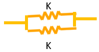
2.
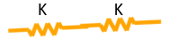
3.
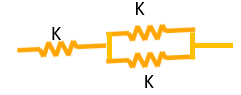
Exercise 3.4: Spring System
Simplify the following system where each spring has a stiffness K.

Exercise 3.4
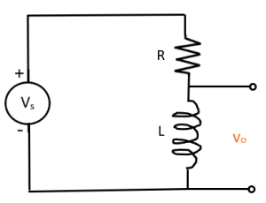
Exercise 3.5
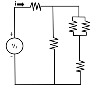
Simplify this circuit into a voltage source and one resistor. Assume all resistors pictured have a resistance R.
Exercise 3.6
Determine the differential equation that models this system.

The right wall has resistance R
All other walls are perfectly insulated
Outside temperature is Ta
A heater is generating a heat flux h
Exercise 3.7: One-Tank Fluid Flow System
 Write a differential equation for the height of the water in the tank.
The tank has a cross-sectional area of A and the outlet has a resistance R.
Media Attributions
- Resistor-470ohm
- DC Motor Position: System Modeling
- File.HCHE.jpg
