
2
2.1 Solving Systems of Differential Equations with LaPlace
Why do we need to know LaPlace Transforms?
In Chapter 1, we focused on representing a system with differential equations that are linear, time-invariant and continuous. These are time domain equations. Through the use of LaPlace transforms, we are also able to examine this system in the Frequency Domain and have the ability to move between these domains of equations.
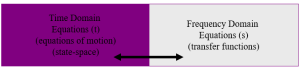
Both domains have certain advantages when trying to understand a system and/or design controllers.
Definition of LaPlace Transforms
The Laplace transform is defined by the equation:
![]()
The inverse of this transformations can be expressed by the equation:
![]()
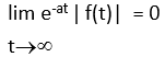
These transformations can only work on certain pairs of functions. Namely the following must be satisfied:
Properties of LaPlace Transforms
Multiplication of a constant: ![]()
Addition: ![]()
Differentiation: ![]()
![]()
Integration: ![]()
Table 2.1 LaPlace Transform Theorems
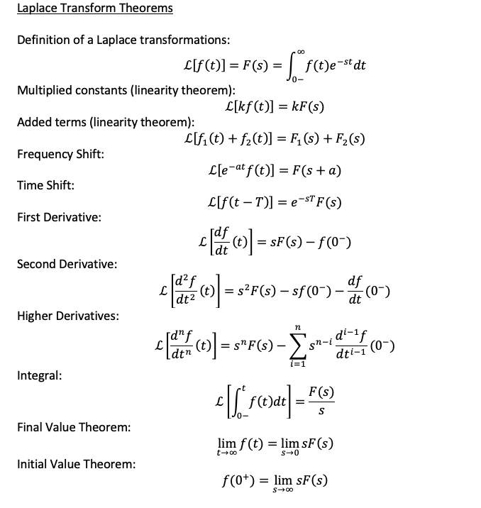
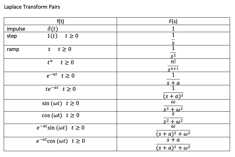
Table 2.2 LaPlace Transform Table
Solving a Differential Equation by LaPlace Transform
1. Start with the differential equation that models the system.
![]()
2. Take LaPlace transform of each term in the differential equation.
3. Rearrange and solve for the dependent variable.
4. Expand the solution using partial fraction expansion.
First, determine the roots of the denominator. Real roots are first-order terms and Imaginary roots are second-order terms.
You can then write the expansion as: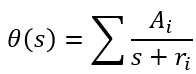
Determine Ai by using partial fraction expansion methods or through the process of combining terms and solving for coefficients.
Any terms with complex roots can be combined with complex conjugates to get a real term that will transform into a sin or cos expression or a combination of these.
5. Take the inverse LaPlace of each term.
![]()
Example 2.1: Solving a Differential Equation by LaPlace Transform
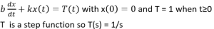
1. Start with the differential equation that models the system.
2. We take the LaPlace transform of each term in the differential equation.
From Table 2.1, we see that dx/dt transforms into the syntax sF(s)-f(0-) with the resulting equation being b(sX(s)-0) for the b dx/dt term. From Table 2.1, we see that term kx(t) transforms into kX(s), and term T(t) transforms into T(s). Recall that T is a step function, so T(s)=1/s.
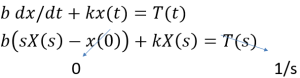
The resulting equation is:
![]()
3. We rearrange the equation to solve for the variable of interest, which in this case is X(s).
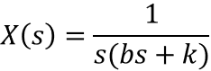
4. Then we factorize the denominator and expand the solution using partial fraction expansion.
![]()
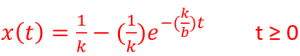
5. Lastly, we determine the inverse LaPlace Transform of each term.
The term ![]() transforms into 1/k and the term
transforms into 1/k and the term ![]() transforms into
transforms into ![]() as shown by Table 2.2.
as shown by Table 2.2.
Partial Fraction Expansion
1. Start with 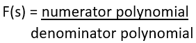 where the highest power of the numerator (m) is less than the highest power of the denominator (n).
2. Factor the denominator polynomial:
![]()
3. If each pole is distinct, the solution can be solved as:
F(s) = a1/(s+p1) + a2/(s+p2) + a3/(s+p3)…
where ai=[(s+pi) F(s)]s=-pi
4. If any poles are multiples (ie. F(s)=(s2+2s+3/(s+1)3) then:
![]() and
and 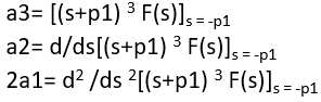
Translating Partial Expansions
F(s)=r1/(s-p1)+r2/(s-p2)+ … rn/(s-pn)
| F(s) | f(t) |
| 1/(s) | 1 |
| 1/(s)2 | t |
| 1/(s+a) | e-at |
| 1/(s+a)2 | t*e-at |
| 1/(s+a)3 | (1/2) t2 *e-at |
| 1/(s+a)4 | (1/6) t3 *e-at |
| … | … |
If complex conjugates are poles:
p1= σ + jω
p2= σ – jω
| F(s) | f(t) |
| w/(s2 + w2) | sin(wt) |
| s/(s2 + w2) | cos(wt) |
| w/((s+a)2 + w2) | e-at sin(wt) |
| (s+a)/((s+a)2 + w2) | e-at cos(wt) |
Solving Partial Fractions in MATLAB
You can solve partial fractions in MATLAB!
residue is a MATLAB function for partial fraction expansion. B(s) is the numerator polynomial and A(s) is the denominator polynomial, as shown below.
F(s)=B(s)/A(s) where B(s)= b0sn+b1sn+…+bn and A(s)=a0sn+a1sn+…+an
When using the residue function, the solution will take the form of: F(s) = r1/(s-p1) + r2/(s-p2) + … +rn/(s-pn) + k(s) where r are the residues and p are the poles.
The MATLAB syntax is shown below:
num = [b0 b1 ... bn];
den =[a0 a1 ... an];
[r,p,k]=residue(num,den)
Information on Matlab’s residue function is available online.
tf2zp is a MATLAB function for converting polynomial transfer functions to zero-pole-gain form. B(s) is the numerator polynomial and A(s) is the denominator polynomial, as shown below.
F(s)=B(s)/A(s) where B(s)= b0sn+b1sn+…+bn and A(s)=a0sn+a1sn+…+an
When using the tf2zp function, the solution will take the form of: F(s) = K[(s-z1) (s-z2) … (s-zn) ]/[(s-p1) (s-p2) … (s-pn)] where z are the zeros, p are the poles and the gains are K.
The MATLAB syntax is shown below:
num = [b0 b1 ….. bn];
den = [a0 a1 ….. an];
[z,p,K] = tf2zp(num, den)
Information on Matlab’s tf2zp function is available online.
Example 2.2
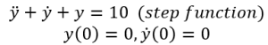
Solve for the output signal y(t).
Recall from Table 2.2 the following transforms for Input Signals: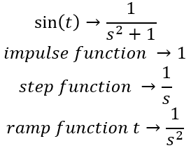
1. Start with the differential equation that models the system. In this example, our input signal will be a step function.
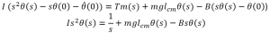
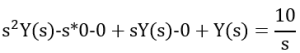
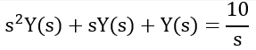
2. Now we take the LaPlace Transform of each term in the differential equation and apply the initial conditions.
![]()
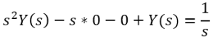
![]()
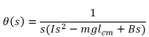
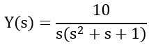
3. Next, we rearrange the equation and solve for the variable of interest.
![]()
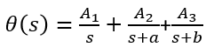
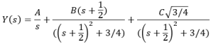
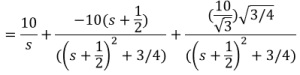
4. Next, we factorize the denominator and expand the solution using partial fraction expansion.
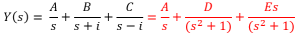
![]()
![]()
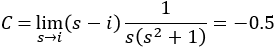
![]()
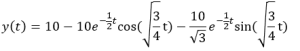
5. Lastly, we find the inverse LaPlace transform of each term.
![]()
What happens if I get complex numbers?
A complex number takes the form A = σ + jω where σ is the real part and ω the imaginary part.
Complex numbers contain the imaginary operator usually denoted as i or j. Recall that j2 = -1 or j=sqrt(-1)
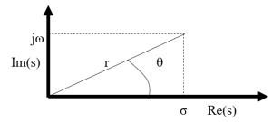
Graphically, these are represented on a plane with the x-axis as the real part and the y-axis as the imaginary part.
A = |A| ∠ θ = r ∠ θ
r = |A| = sqrt(σ2+ω2)
θ=tan-1(ω/σ)
Recall that for the Complex Conjugate of a complex number, you take the initial complex number and change the sign for the imaginary part.
A*=σ – jω
AA*=(|A|)2
Euler’s Theorem
A=cosθ + j sinθ = eiθ
dA/dθ= -sinθ + j cosθ = j2 sinθ + j cosθ = j ( j sinθ + cosθ) = j A
dA/dθ = j A → dA/A = j/dθ
∫ dA/A = ∫ j/dθ → ln A = j θ + c
A= e(j θ + c)
Since |A|=1 and when the imaginary part is zero, θ=0, therefore c=0
A = cosθ + j sin θ = e j θ A* = cosθ – j sin θ = e-j θ
cos θ = 1/2 (e j θ + e -j θ ) sin θ = 1/2j (e j θ – e -j θ )
Example 2.3
1. Start with the differential equation that models the system. In this example, our input signal will be a step function.
2. Now we take the LaPlace Transform of each term in the differential equation and apply the initial conditions.
3. Next, we rearrange the equation and solve for the dependent variable.
4. Next, we factorize the denominator and expand the solution using partial fraction expansion.
5. Lastly, we find the inverse LaPlace transform of each term.
2.2 Transfer Functions
If we set both the input signal and the output signal as variables in the LaPlace space and set initial conditions to zero, we can solve for one of the output conditions to get a transfer function for the system:
O(s)/I(s)=TF(s)
where O(s) is the output, I(s) is the input, o(t)=0 and do/dt=0
For this approach, we:
1. Start with the differential equation, assume initial conditions are zero or adjust variable to have zero initial conditions.
![]()
2. Take the LaPlace Transform.
![]()
3. Using algebra, solve for the Transfer Function by dividing the variable of interest by the input signal in LaPlace space.
![]()
4. Use the resulting Transfer Function to understand the system and design controllers.
For Transfer Functions,
- The system should be linear (often linearized around an equilibrium point, so initial conditions are zero).
- The system should be time invariant.
- The system should be single input, single output.
With transfer functions, we can use block diagrams, signal flow diagrams or Bond graphs, although this textbook will generally focus on use of block diagrams, as discussed in Chapter 4.
Getting the System Behavior
You can solve for the output signal as a function of time by:
1. Multiplying by the input signal: ![]()
2. Taking the inverse LaPlace: ![]()
Although, we don’t always have to solve for the output signal. Knowing about potential solutions, we can get a pretty good idea of the solution just from the Transfer Function. This is discussed in more depth in Chapter 4.
Introduction to Poles and Zeros and Zero-Pole-Gain Representation
Recall that Transfer Functions are represented in this form:
TF(s)=O(s)/I(s)
where O(s) is the output and I(s) is the input.
After a system has been represented by a Transfer Function, the numerator and denominator can be factorized, resulting in Zero-Pole-Gain Representation.
F(s)=K[(s-z1) (s-z2) … (s-zn) ]/[(s-p1) (s-p2) … (s-pn)]
Zeros, denoted as z, are roots of the numerator. Poles, denoted as p, are roots of the denominator. K is the system Gain.
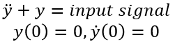
Example 2.5
![]()
We generally work with the assumption that initial conditions are zero: y(0)=0, ÿ(0)=0
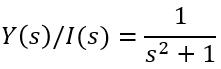
Identify the output signal: Y(s)
Identify the input signal: I(s)
Using Table 2.1, the resulting equation from the LaPlace Transform is:
s2Y(s)+Y(s)=I(s)
Solve for the Transfer Function by performing output/input: Y(s)/I(s)
A Transfer Function is not a signal, so you wouldn’t take the inverse LaPlace without first multiplying it by a signal.
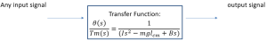
Example 2.6
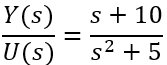
Determine the Transfer Function Y(s)/U(s)
![]()
Assumption: initial conditions are zero.
Using Table 2.1, the resulting equation from the LaPlace Transform is:
![]()
Solve for the Transfer Function by performing output/input: Y(s)/I(s)
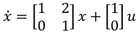
Going from State-Space to Transfer Functions
To go from State-Space to Transfer Function, we first need to identify the four matrices A, B, C and D:
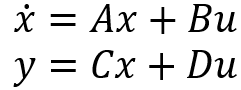
Recall that for Transfer Functions, the system must be linear, time invariant, and SISO (single input, single output).
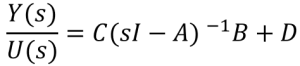
Or, we can go back to the differential equations, take the LaPlace Transform, and then form the Transfer Function.
Example 2.7
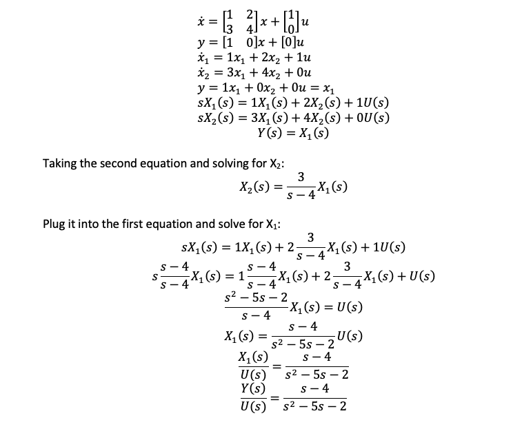
In Matlab, this answer can be checked with the following code:
B = [1;0];
C = [1 0];
D = 0;[num, den] = ss2tf(A,B,C,D);
sys = tf(num,den);
sys =
s – 4
————-
s^2 – 5 s – 2
System Representation in MATLAB
Systems can be represented as:
1. Transfer Function
Transfer Function – numerator and denominator polynomials
F(s)=O(s)/I(s)
F(s)=[b0sn+b1sn+…+bn]/[a0sn+a1sn+…+an]
Zero, Pole Transfer Function – z(zeros), p(poles), K
F(s)=K[(s-z1) (s-z2) … (s-zn) ]/[(s-p1) (s-p2) … (s-pn)]
2. State-Space (linear)
State-Space – matrices A, B, C, D
dx/dt= Ax(t)+Bu(t)
y=Cx(t)+Du(t)
where zeros = [z0 z1 ….. zn], num = [b0 b1 … bn], A=[1 0;0 1], B = [1;0], poles = [p0 p1 ….. pn], den = [a0 a1 … an]; C=[1 0]; D=0.
In MATLAB, the following commands zpk, tf, and ss relate to zero-pole gain model, transfer function model, and state-space model respectively.
sys = zpk(z,p,K),
sys = tf(num, den),
sys = ss(A,B,C,D).
Converting between systems can be done with the following MATLAB commands:
- tf2zp – transfer function to zero-pole
- tf2ss – transfer function to state-space
- zp2ss – zero-pole to state-space
- zp2tf – zero-pole to transfer function
- ss2tf – state-space to transfer function
- ss2zp – state-space to zero-pole
Other functions that may be useful:
- step – returns the response of a system to an input signal of a unit step
- impulse– returns the response of a system to an input signal of a unit impulse
Exercises
Exercise 2.1
Solve the Differential Equation by LaPlace Transform.
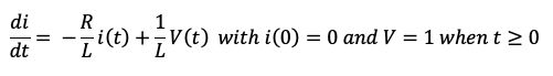
Where R=1, L=1 and V is a step function, so V(s)=1/s
Exercise 2.2
Determine the Transfer Function Y(s)/I(s)
![]()
Exercise 2.3
Determine the Transfer Function.
![]()
Media Attributions
- chapter2_integral
- Laplacetheorems
- laplacetable
- Screen Shot 2020-08-17 at 8.48.55 PM
- Screen Shot 2020-08-17 at 8.58.12 PM
