7
6.1 Frequency Response
Recall from previous chapters our focus on Transient Response.
![]()
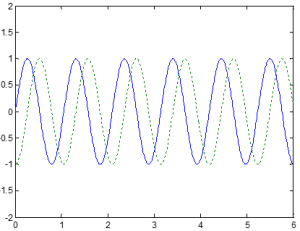
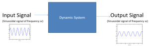
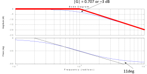
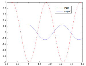
Frequency Response allows for us to investigate the steady-state response of a system with a sinusoidal input. The response is expected to be a sine wave of the same frequency, but may be offset in time and have a different magnitude.
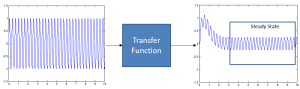

In the plot to the left, we have plotted the sinusoidal input and output signals of a system.
The input signal is represented by the equation I=Ai sin(ωt+θ) where Ai is the amplitude of the input signal, ω is angular frequency, and θ is the angle that the waveform has been shifted, if applicable.
The output signal is represented by the equation I=Ao sin(ωt+θ+ø) where Ao is the amplitude of the output signal, ω is angular frequency, θ is the angle that the waveform has been shifted, if applicable, and ø is phase.
The magnitude is defined as M=Ao/Ai and phase is defined as ø=(Δt/T * 360º).
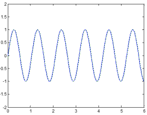
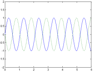
For the example plots below, the blue line indicates the input signal and the green line indicates the output signal. Based on these signals, we can determine the magnitude.
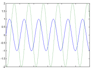
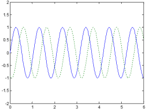
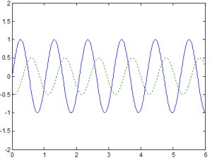
For the example plots below, the blue line indicates the input signal and the green line indicates the output signal. Based on these signals, we can determine the phase.
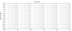
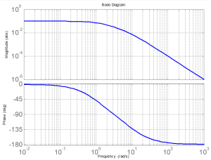
6.2 Bode Plots
One can plot the Magnitude and Phase as a function of the input frequency; this is a Bode Plot.
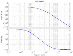
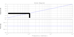
As shown below, the top plot is Magnitude versus frequency. The bottom plot is Phase versus frequency. Magnitude and Frequency are commonly measured on a logarithmic scale, although Magnitude can also be transformed into decibels (dB) and plotted on a linear scale.
In order to plot Magnitude on a linear scale, it can be transformed into decibels (dB) using the following equation: ![]()
This relationship can be seen in the following graphs:
Ways to Get Bode Plots
1. Experimental Data
We can use Experimental Data to sketch Bode Plots.
Test 1: Frequency: w1 → M1, ø1
Test 2: Frequency: w2 → M2, ø2
Test 3: Frequency: w3 → M3, ø3
Test 4: Frequency: w4 → M4, ø4
Test 5: Frequency: w5 → M5, ø5
2. Calculating Magnitude and Phase
Direct Calculation Method:
1. Start with the Transfer Function
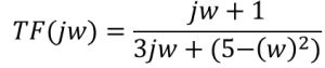
2. Substitute s= jw
3. For both the numerator and denominator, isolate the real and imaginary parts:
![]()
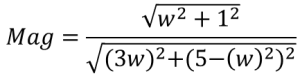
4. Calculate the magnitude and phase data:
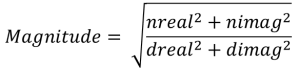
![]()
5. Do this for each value of w
3. Using Bode Drawing Techniques
Construction Technique:
First, rewrite the given transfer function into first and second-order terms.
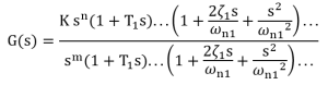
or by substituting s=jw into the equation:
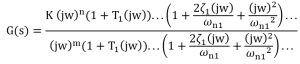
The table below details the trends for plotting the magnitude and phase approximation for each term of the transfer function:
| Term | Magnitude (dB) | Phase |
|---|---|---|
| K | 20 logK | no phase change |
| jwn | 20*n dB/decade crossing 0 dB at w=100=1 | n*90 degrees |
| (1+T(jw))n, n=±1 | 20*n dB/decade starting at w=1/T | n*90 degrees starting at w=1/T |
 , n=±1 , n=±1 |
40*n dB/decade starting at w=ωn | n*180 degrees starting at w=ωn |
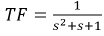
Example 6.1
Get the Bode Plot from the Transfer Function using the Direct Calculation Method.
1. Start with the Transfer Function
2. Substitute s= jw

3. For both the numerator and denominator, isolate the real and imaginary parts:
4. Calculate the magnitude and phase data:

5. Do this for each value of w
Bode Plot for a Constant
G(s)=K
where Magnitude = 20 log10K and Phase = 0 degrees.

Bode Plot for a Zero/Pole at the Origin
For jwn, the magnitude has a slope of 20*n dB/decade crossing 0 dB at w=100=1. The phase is a horizontal line at n*90 degrees.
The Bode Plot for G(s)=s is shown below:
where the slope of the Magnitude is 20 dB/decade going through (1 rad/s, 0 dB) and the Phase is 90 degrees.
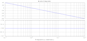
The Bode Plot for G(s)=1/s is shown below:

where the slope of the Magnitude is -20 dB/decade going through (1 rad/s, 0 dB) and the Phase is -90 degrees.
The Bode Plot for G(s)=s2 is shown below:

where the slope of the Magnitude is 40 dB/decade going through (1 rad/s, 0 dB) and the Phase is 180 degrees.
The Bode Plot for G(s)=1/s2 is shown below:
where the slope of the Magnitude is -40 dB/decade going through (1 rad/s, 0 dB) and the Phase is -180 degrees.
Bode Plot for a Real Negative Zero/Pole
For (1+T(jw))n, n=±1, the magnitude has a slope of 20*n dB/decade starting at w=1/T. The phase is a horizontal line at n*90 degrees starting at w=1/T.
The Bode Plot for G(s)=Ts+1 is shown below:

For T=1 in this example, the slope of the Magnitude is 20 dB/decade at w=1/T and the Phase is 90 degrees at w=1/T.
The Bode Plot for G(s)=1/(Ts+1) is shown below:
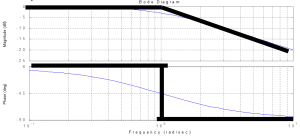
For T=1 in this example, the slope of the Magnitude is -20 dB/decade at w=1/T and the Phase is -90 degrees at w=1/T.
Bode Plot for Complex Negative Poles/Zeros
For, n=±1, the magnitude has a slope of 40*n dB/decade starting at w=ωn. The phase is a horizontal line at n*180 degrees starting at w=ωn.
The Bode Plot for ![]() is shown below:
is shown below:

For ωn=1 in this example, the slope of the Magnitude is 40 dB/decade at w=ωn1 and the Phase is 180 degrees at w=ωn1.
The Bode Plot for  is shown below:
For ωn=1 in this example, the slope of the Magnitude is -40 dB/decade at w=ωn1 and the Phase is -180 degrees at w=ωn1.
Creating a Bode Plot
1. Rewrite the given transfer function into first and second-order terms.
2. Plot each element approximation for Gain, s terms, poles, zeros, complex poles, complex zeros, etc.
3. Round off corners.
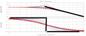
First-Order:
At the break point (ω), which is where the two asymptotes meet, the corner will be rounded off. The Magnitude at a break point is off by 3 dB. In the example below, the magnitude curve would occur below the break point by -3 dB, resulting in a rounded corner. If at the breaking point, the slope following the point was positive, the magnitude curve would occur above the break point by 3 dB.
As shown above, the Phase at the break point is -45 degrees.
Second-Order:
4. Add the plots together, if Magnitude is measured in dB, or multiply Magnitude plot if on logarithmic scale.
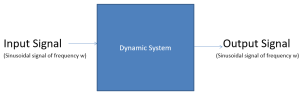
6.3 Frequency Response Control Design
6.4 Adjusting Gain and Phase Margin
6.5 Adjusting Steady-State Error
6.6 Nyquist Plots
Exercises
Exercise 6.1
What is the magnitude (dB), phase shift (degrees) and frequency (rad/s) of this output relative to the input?
Exercise 6.2
Get the Magnitude (dB) and Phase for all values of w for the following transfer function:
Exercise 6.3
Sketch the Bode Plot of the transfer function:

Exercise 6.4
Sketch the Bode Plot of the Transfer Function: