
4
4.1 Utilizing Transfer Functions to Predict Response
Review from Chapter 2 – Introduction to Transfer Functions
Recall from Chapter 2 that a Transfer Function represents a differential equation relating an input signal to an output signal. Transfer Functions provide insight into the system behavior without necessarily having to solve for the output signal.
Recall that Transfer Functions are represented in this form:
TF(s)=O(s)/I(s)
where O(s) is the output and I(s) is the input.
After a system has been represented by a Transfer Function, the numerator and denominator can be factorized, resulting in Zero-Pole-Gain Representation.
F(s)=K[(s-z1) (s-z2) … (s-zn) ]/[(s-p1) (s-p2) … (s-pn)]
Zeros, denoted as z, are roots of the numerator. Poles, denoted as p, are roots of the denominator. K is the Gain.
You can solve for the output signal as a function of time by:
1. Multiplying by the input signal: ![]()
2. Taking the inverse LaPlace: ![]()
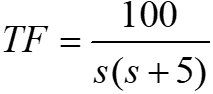
Predicting Response through Pole Location
Instead of using inverse LaPlace to determine the response, you can use pole locations from the Transfer Function to predict the response!

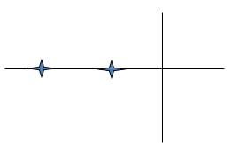
1. Start by taking the denominator of the transfer function and set it equal to zero. This is the the characteristic equation. Determine the roots of the characteristic equation. These are the poles.
![]()
If the poles are real, you would expect a term like this to be in the response:
![]()
If the poles are imaginary, you would expect a term like this to be in the response:
![]()
If the poles are complex, would expect a term like this to be in the response:![]()
2. Plot on Re-Im plane.

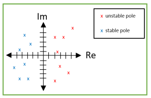
If the real part of the pole is negative, then the system is stable. Location of the poles predicts behavior.
Note: In state-space, the eigenvalue equation gives you the characteristic equation: det(sI-A)=0 and the eigenvalues are the poles.
Example 4.1:
The transfer function and state-space are for the same system.


From the transfer function, the characteristic equation is s2+5s=0, so the poles are 0 and -5.
For the state-space, det(sI-A)= ![]() = (s2+5s)-(1*0) = s2+5s=0, so the poles are 0 and -5.
= (s2+5s)-(1*0) = s2+5s=0, so the poles are 0 and -5.
Both yield the same answer as expected.
Graphing the Response
Below are graphs demonstrating the trends of the response to an input step signal:

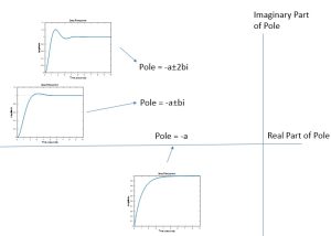
Why are these the trends?
For oscillation, notice that a pole along the Real axis doesn’t cause the response to oscillate. As the pole moves along the Imaginary axis, the frequency of oscillation increases. Notice that as a pole moves away from zero on the Real axis, the response settles more quickly. Also notice that a pole to the right of the Imaginary axis causes for the system to be unstable!
Solved Responses of Systems
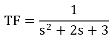
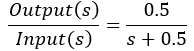
Using the denominator of the transfer function, we can use the power of s to determine the order of the system.
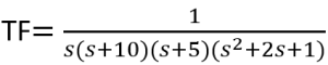
For example, in the given transfer function  , the power of s is two in the denominator term, meaning that this system is a second-order system.
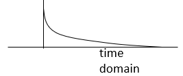
An impulse input results in an impulse response of the system. A step input results in a step response of the system. A ramp input results in a ramp response of the system.
First Order System
TF=1/(Ts+1)
| Impulse Response | Step Response | Ramp Response |
|---|---|---|
| output signal = (TF)(1) | output signal = (TF)(1/s) | output signal = (TF)(1/s2) |
| O(s) = 1/(Ts+1) → o(t) = (1/T) e–t/T | O(s) = 1/[s(Ts+1)] → o(t) = 1- e-t/T | O(s) = 1/[s2 (Ts+1)] → c(t) = t – T + e-t/T |
| Output signal plot
What is the impulse function?
Recall that δ(t) represents a unit impulse signal. δ(t) = 1/ε when δ(t) = 0 when It is typically used in continuous systems. ∫δ(t) dt = 1 For LaPlace Transform, δ(s) = 1 |
Output signal plot
What is the step function?u(t) = 1 when t(t) = 0 when t<0
|
Output signal plot
steady state solution c(t) = t-T steady state error = r(t)-c(t) = t-(t-T) =T
What is the ramp function?u(t) = t when t(t) = 0 when t<0
|

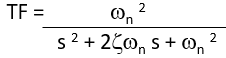
Second Order System
TF = 1/(Is2 + Bs + K)
To find the poles of this transfer function, we can use the quadractic formula:
![]()
![]()
If (B/2I)2 – (K/I) ≥ 0 then there are 2 real poles.
If (B/2I)2 – (K/I) < 0 then there are 2 complex conjugate poles.
Defining terms in the quadratic equation:
K/I = ωn2
B/I = 2ζωn = 2σ
where ωn is the natural frequency, ζ is the damping ratio, and σ is attenuation.
Step Response of a Second Order System
Recall for a step input, C(s)=TF(s)*1/s where C(s) is the output and TF(s) is the transfer function and 1/s is the step input.
| Damping Ratio | Response when t > 0 |
|---|---|
| underdamped (0 < ζ < 1) | |
| critically damped (ζ = 1) | |
| overdamped (ζ > 1) |
Impulse Response of a Second Order System
Recall for an impulse input, C(s)=TF(s)*1 where C(s) is the output and TF(s) is the transfer function and 1 is the impulse input.
| Damping Ratio | Response when t > 0 |
|---|---|
| underdamped (0 < ζ < 1) |  |
| critically damped (ζ = 1) | |
| overdamped (ζ > 1) | |
| undamped (ζ=0) |
When a second-order system is underdamped, there are two roots that are complex conjugates. When a second-order system is critically damped, there are two real and equal roots. When a second-order system is overdamped, there are two real and unequal roots. When a second-order system is undamped, there are two imaginary roots.
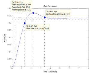
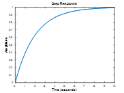
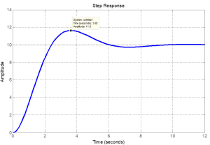
4.2 Transient Response Characteristics
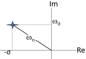
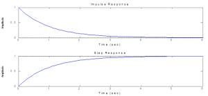
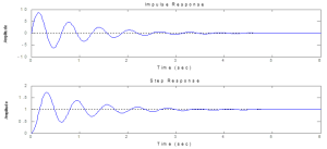
The Rise Time (tr) is 1.04 seconds. This is the time duration from 10% of the final value to 90% of the final value.
tr ≈ 1.8/wn
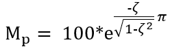
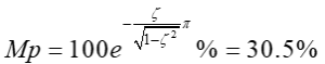
As shown in the figure, the peak amplitude, also known as the maximum, is 0.369. The final value is approximately 0.333.
 This is the Maximum Overshoot (Mp), which is usually expressed as a percent.
Peak time (tp) is the duration it takes to reach the maximum amplitude. This is 2.2 seconds.
tp=π/ωd
The Settling Time (ts), as indicated by the figure, is 3.4 seconds. This is the time it takes for the response to settle to the final value within a certain margin of error.
For 2% criterion, ts = 4/(ζωn)
For 5% criterion, ts = 3/(ζωn)
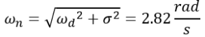
ωn is the natural frequency, ζ is the damping ratio, σ is attenuation, and ωd is the damped natural frequency, where ![]() and σ=ζωn.
and σ=ζωn.
Steps to Pole Location
1. Determine the differential equation of the SISO system.
2. Determine the Transfer Function.
3. Take the denominator of the transfer function and set equal to zero. Solve for the poles.
![]()
![]()
4. Plot the poles on the Real-Imaginary plane.

5. Determine the stability and step response dynamics.

Damping ratio = σ/ωn = 0.35
2% settling time = 4/σ = 4/1
System Identification
First Order or more – at least one real pole
Second Order or more – at least two complex poles
Log-decrement Method

The Log-decrement Method is used to examine impulse and step responses.
y=Ae-at
Decrement (δ) = ln (y0/y1) = a td → a = δ/td
Example 4.2: Impulse Response of a Second-Order System

e-σt sin(ωd t)
For the term e-σt : Decrement (δ) = ln (y0/y1) = σ td → σ = δ/td
For the term sin(ωd t): td = 2π/ωd → ωd = 2π/td
Additionally, we know σ = ζ ωn and ![]() , so
, so
ωn2= ωd2+ σ2
By solving for σ and ωd, we can determine the denominator (s2 + 2ζωn s + ωn2 ) and poles (– σ ± ωd i)
In conclusion, given an impulse response, we can calculate frequency and decay, and get the constants of the denominator.
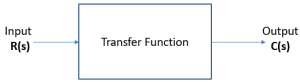
4.3 Block Diagrams
Block diagrams provide a graphical way to represent and solve transfer functions.
Elements of Block Diagrams
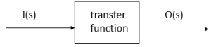
Block

O(s) = G(s) I(s)
where G(s) is a transfer function, O(s) and I(s) are signals.
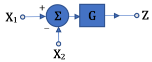
Summing Point
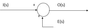
O(s) = I(s) + E(s)
where O(s), I(s) and E(s) are signals.
Branch Point

O(s) = O(s) = O(s)
where O(s) is a signal.
Properties of Block Diagrams
Series
Series blocks are multiplied.

B(s) = R(s)G(s)
C(s) = H(s)B(s) = G(s)H(s)R(s)
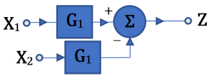
Parallel
Parallel blocks are added.
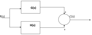
C(s) = R(s)G(s) + H(s)R(s) = (G(s)+H(s))R(s)
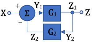
Feedback Loop

where G(s) and H(s) are transfer functions.
Open-Loop Transfer Function
B(s) = G(s)H(s)E(s) → B(s)/E(s) = G(s)H(s)
Feedforward Transfer Function
C(s) = G(s)E(s) → C(s)/E(s) = G(s)
Closed-Loop Transfer Function
C(s) = G(s)E(s)
E(s) = R(s) – B(s) = R(s) – C(s)H(s)
C(s) = G(s) (R(s) – C(s)H(s))
C(s) (1+G(s)H(s)) = G(s)R(s)
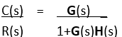
This represents negative feedback.
If feedback is positive, the sign in the denominator changes:

Rules for Block Diagrams
- Product along a path from input to output remain the same.
- Products around a loop remain the same.
- Inner loops should be solved first.
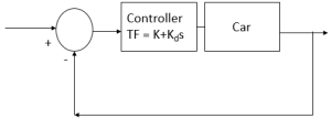
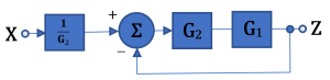
Example 4.3
Feedforward TF:
Openloop TF:
Closedloop TF:
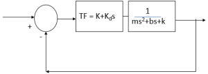
Example 4.4 : Cruise Control
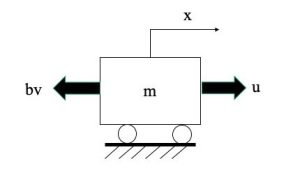
Variables:
Input:
Output:
Transfer Function:
Feedforward TF:
Openloop TF:
Closedloop TF:
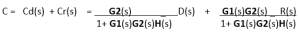
More than one input signal
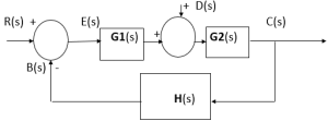
Determine the function for the disturbance:
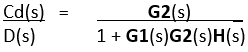
Determine the function for the signal:
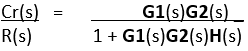
The complete transfer function for this system:
Simplifying Techniques

![]()
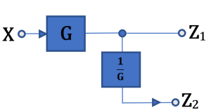
![]()
![]()
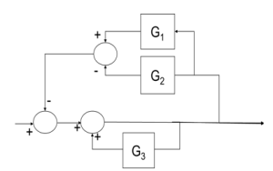
Example 4.5
Simplify the block diagram below.

The loop containing G1 and G3 results in positive feedback, so the block diagram simplifies to be the following:
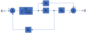
And by following the first simplification technique, the system is simplified to:

4.4 More on Poles
For systems with more than two poles, the pole farthest to the right will be dominant. You may see some influence of other poles in the overall behavior, but we will focus on the one furthest to the right.
4.5 Stability
Determining Stability through Pole Locations
A Linear Time Invariant system is considered stable if the poles of the transfer function have negative real parts. If even one of the poles has a positive real part, then the system is unstable. This means that a pole on the left-hand side of the Imaginary axis is stable and a pole on the right-hand side of the Imaginary axis is unstable.
Determining Stability through use of Phase-Plane Plot
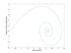
Recall the following from Matlab Example 1.1 in Chapter 1:
The differential equation representing a slightly damped inverted pendulum is as follows:
![]()
We know the initial conditions of the state variables.
We examined a phase plane plot, which is a plot of one state variable against another state variable, in this example, the angular velocity versus the angle:
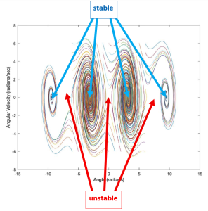
Additionally, we examined the system dynamics for an array of initial conditions:

Determining Stability through Energetics
Potential Energy, as a function of state variables, is a surface that defines stability.

The first derivative of potential energy defines equilibria:

The second derivative of potential energy defines stability:

One can think about potential energy as a ball on a hilly surface.
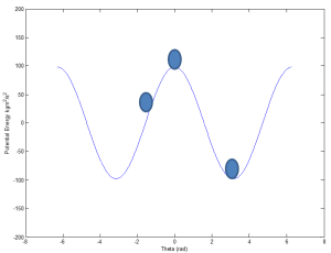
Where can the ball settle/balance? This is equilibrium.
When in equilibrium, what might happen what a slight perturbation?
How might one describe this mathematically?
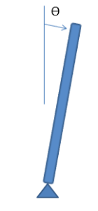
Example 4.6: Is an inverted pendulum stable without a motor?
The following differential equation represents the system:
![]()
The potential energy for the system can be represented as:
![]()
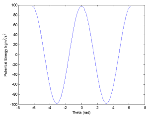
Given the equation for the potential energy (V) of an inverted pendulum without a motor:
![]()
.
.
We take the first derivative of the potential energy (V) equation to define the equilibria:
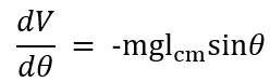
Then we take the second derivative of potential energy to define stability:
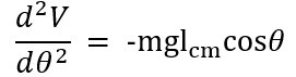
For small angles, we approximate θ=0, so our equations become:
![]()
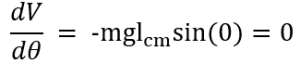
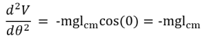
Due to the second derivative of potential energy resulting in a value less than zero, the system is unstable.
What if we added a spring to the inverted pendulum?
Here is the equation for the potential energy (V) of an inverted pendulum with a spring:

We take the first derivative of the potential energy (V) equation to define the equilibria:

Then we take the second derivative of potential energy to define stability:
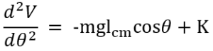
For small angles, we approximate θ=0, so our equations become:

This means that if K-mglcm > 0, then the system is stable.
4.6 Steady-State Values
We can use the following identity to find the steady state function of a response:
TF(s)=C(s)/R(s) → C(s)=TF(s)*R(s)
The Final Value Theorem can be used to determine the response of the system as time approaches infinity:
![]()
where R(s) is the input, C(s) is the output, and TF(s) is the transfer function.
For a step response: ![]()
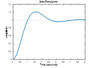
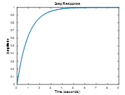
Example 4.7
Apply the Final Value Theorem to determine the response of the system as time approaches infinity.

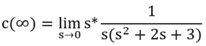
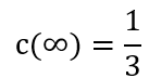
The resulting steady-state value to unit step input is 0.333 and can be seen on the plot as well.
Exercises
Exercise 4.1
Match the response to the transfer function. All plots are on the same time scale.


Exercise 4.2
For the following complex poles, what do you predict the settling time to be?
b. pole = -50
c. poles = 25±6i
Exercise 4.3
What are the expected overshoots of a step response for the following:

Exercise 4.4
For the following step response, fill in the red blanks for the expected response dynamics: e_sin(_t)

What are the two complex poles and what could the transfer function be?
Exercise 4.5
Simplify the block diagram.
Exercise 4.6
What are the steady-state values of a step response for the following transfer functions:


![]()
Exercise 4.7
What is the steady-state value of these step responses?
Media Attributions
- Screen Shot 2020-09-28 at 2.41.14 PM
